03 - Model interpretability, filters and features visualization

Advanced Image Processing

Poznan University of Technology, Institute of Robotics and Machine Intelligence

Laboratory 3: Model interpretability, filters and features visualization

Introduction

In this laboratory, you will learn how to peek inside the “black box” of deep neural networks to understand their decision-making processes. We’ll move beyond just measuring accuracy and explore the crucial field of model interpretability.

You will get hands-on experience with two key techniques:

visualization of filters - you’ll learn how to inspect the convolutional filters of a trained model to see the fundamental patterns and textures they have learned to detect, from simple edges and colors in early layers to more complex shapes in deeper ones
visualization of features - we will examine the feature maps (or activation maps) to see how the model “views” a specific input, highlighting which areas of an image it focuses on to make its prediction

To achieve this, we will be using Captum, a powerful and flexible open-source library from PyTorch. Captum provides a unified interface to state-of-the-art attribution algorithms, allowing you to easily calculate and visualize which input features are most responsible for a model’s output, helping you debug, validate, and build trust in your AI systems.

Goals

The objectives of this laboratory are to:

learn how to inspect the convolutional filters of a trained model,
explore interpretability algorithms for computer vision models and learn how to visualize their output (activation map),
familiarize with Captum package.

Prerequisites

Install dependencies

PyTorch

pip3 install torch torchvision --index-url https://download.pytorch.org/whl/cu126

Lightning

pip install lightning

Import libraries

import json

from matplotlib import pyplot as plt
import numpy as np
import requests
import torch
import torch.nn.functional as F
from torchvision import models
from torchvision import transforms
from PIL import Image

Load pretrained model and labels

In this step, we’ll load a powerful, off-the-shelf image classification model called ResNet-34. A pretrained model is like a seasoned expert who has already studied millions of examples. 🧠 This specific model is a deep convolutional neural network with 34 layers that has already been trained on the massive ImageNet dataset.

ImageNet is a famous computer vision dataset containing over 14 million images, each hand-labeled into one of 1000 distinct categories (e.g., “golden retriever”, “strawberry”, “space shuttle”). By using a model pretrained on this data, we leverage a vast amount of learned knowledge about visual features right from the start.

Alongside the model, we’ll also load the corresponding list of ImageNet’s 1000 class labels. This is crucial because the model outputs its prediction as an index number (e.g., 159), and we need this list to map that number to a human-readable name (e.g., “Rhodesian ridgeback”).

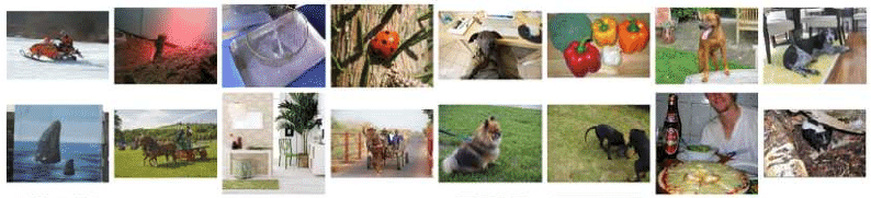
Sample images from ImageNet-1K database. Image source: Multipod Convolutional Network

💥 Task 1 💥

Based on Models and pre-trained weights documentation load ResNet-34 model with IMAGENET1K_V1 weights. Set the model to evaluation mode.

To load ImageNet class labels used the following code:

# Download ImageNet class labels
labels_url = "https://s3.amazonaws.com/deep-learning-models/image-models/imagenet_class_index.json"
response = requests.get(labels_url)
labels = response.json()
labels = {int(k):v[1] for k,v in labels.items()} # Convert keys to integers and get the label name

Model utility functions

Deep learning models usually require data in a specific tensor format. Therefore, to correctly communicate with our model, we need two helper functions:

Pre-processing - transforms raw input data into a clean, standardized, and numerical format that a deep learning model can efficiently and effectively understand. This often includes steps like resizing an image to a fixed dimension (e.g., 224×224 pixels), normalizing pixel values, and converting the data into a tensor.
Post-processing - converts the raw, numerical output of a deep learning model into a final, interpretable format, such as assigning a class label or drawing bounding boxes on an image.

These utilities handle the crucial tasks of transforming our input image into a valid tensor and converting the model’s raw output back into an understandable prediction.

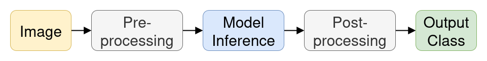
Model inference pipeline for image classification.

############# TODO: Student code #####################

# ImageNet-based pre-processing image transformations
transform = transforms.Compose([
    ...
])

######################################################


def preprocess_image(img: np.ndarray) -> np.ndarray:
    """Preprocesses an image for model inference."""
    input_tensor = transform(img)
    input_tensor = input_tensor.unsqueeze(0) # Add batch dimension
    return input_tensor


def postprocess(output: torch.Tensor, labels: dict[int, str]) -> tuple[str, int, float]:
    output = F.softmax(output, dim=1)
    prediction_score, pred_label_idx = torch.topk(output, 1)
    pred_label_idx.squeeze_()
    predicted_label = labels[pred_label_idx.item()]
    return predicted_label, pred_label_idx, prediction_score.item()

💥 Task 2 💥

Using transforms.Compose, write a model input transformation pipeline that follows the ImageNet preprocessing steps. The pipeline should consist of the following methods in this order: 1. Resize to scale image into 256x256 resolution 2. CenterCrop to crop the given image at the center, with size=224 3. ToTensor 4. Normalize with mean=[0.485, 0.456, 0.406] and std=[0.229, 0.224, 0.225]

ImageNet-based transforms for pre-trained model.

Inference pre-trained model

############# TODO: Student code #####################

img_url = "https://images.pexels.com/photos/20816519/pexels-photo-20816519.jpeg"
img = Image.open(requests.get(img_url, stream=True).raw)

predicted_label = -1
prediction_score = 0.0

######################################################

fig = plt.figure(figsize=(8, 5))
plt.imshow(img)
plt.title(f"Predicted class: '{predicted_label}' with confidence {prediction_score:.2f}")
plt.axis('off')
plt.show()

💥 Task 3 💥

Write model inference code that follows the sequence presented in model inference graph. Test this pipeline on different images.

Model layers inspection

To understand what’s happening inside our model and how it is constructed, we can examine its entire architecture. This process is like creating a detailed blueprint or an X-ray of the neural network, showing every layer and the connections between them. To do this we can use online tools like Netron or packages like PyTorchViz.

To install PyTorchViz from the command line interface call:

pip install torchviz

To save a model graph to a file use the following code snippet:

from torchviz import make_dot


# Create a dummy input tensor
dummy_input = torch.randn(1, 3, 224, 224)

# Perform a forward pass to get the output tensor
output = model(dummy_input)

# Generate the graph visualization
# We visualize the output tensor and specify the model's parameters for a clearer graph.
dot = make_dot(output, params=dict(model.named_parameters()))

# Save the graph to a file (e.g., PDF, PNG)
dot.render("resnet34_torchvision_graph", format="png", cleanup=True)

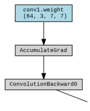
Part of the generated model graph.

💥 Task 4 💥

Inspect ResNet-34 model graph, saved as resnet34_torchvision_graph.png. Familiarize yourself with the convention for naming convolutional layers - it will be useful for the next task.

Model understanding - visualization of convolutional filters

One of the best ways to understand what a Convolutional Neural Network (CNN) has learned is to peek inside and look at its convolutional filters. Think of these filters as the fundamental building blocks of the model’s vision. Each filter is a small kernel trained to detect a very specific, low-level feature in an image.

In the early layers of the network, these features are incredibly simple, like horizontal or vertical edges, specific colors, gradients, or simple textures. As you go deeper into the network, subsequent layers learn to combine these simple patterns into more complex concepts, like eyes, wheels, or fur.

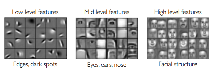
Features hierarchy. Image source: introtodeeplearning.com

In this section, we’ll extract the weights from the very first convolutional layer of our ResNet-34 model and visualize them. This allows us to see the most basic patterns the network is looking for, providing a fascinating glimpse into how it begins to deconstruct and understand the visual world. It’s the first step in moving the model from a “black box” to something more interpretable.

def postprocess_filter(img_tensor: torch.Tensor):
    """Helper function for post-processing and display."""
    img = img_tensor.squeeze(0).cpu().detach().numpy()
    img = np.transpose(img, (1, 2, 0))
    # Normalize to [0, 1] for display
    img = (img - img.min()) / (img.max() - img.min())
    return img


def visualize_filter(model, layer: str, filter_index: int, iterations: int = 50, lr: float = 0.1) -> np.ndarray:
    """Generates an image that maximally activates a specified filter."""
    # Start with a random noise image (our canvas)
    image = torch.randn(1, 3, 224, 224, requires_grad=True)
    optimizer = torch.optim.Adam([image], lr=lr, weight_decay=1e-6)

    # We need to hook into the model to capture the output of our target layer
    activation = None
    def hook(model, input, output):
        nonlocal activation
        activation = output

    handle = layer.register_forward_hook(hook)

    print(f"Computing Filter #{filter_index} of layer {layer.__class__.__name__}...")
    for i in range(iterations):
        optimizer.zero_grad()
        # Forward pass to get the activation
        model(image)
        # Our "loss" is the negative of the mean activation of the chosen filter.
        # We negate it because optimizers minimize, but we want to maximize.
        loss = -torch.mean(activation[0, filter_index])
        loss.backward()
        optimizer.step()

    handle.remove() # Clean up the hook
    return postprocess_filter(image)

💥 Task 5 💥

Compute any three convolution filters for early, middle and late layers filters. For example for the following layers:

layer1[0].conv1 (Early Layer Filters)
layer3[0].conv2 (Middle Layer Filters)
layer4[1].conv1 (Late Layer Filters)

Visualize them in a single graph (3x3 grid, with filter number in subplot title) and answer the following questions:

In your own words, describe the evolution of the patterns from the early, to the middle, and finally to the late layers. How does the complexity change?
Look at the three filters you visualized from a single layer (e.g., the early layer). Did they all detect the same pattern? Why is it crucial for a network to have filters that specialize in different patterns within the same layer?
Explain how this learned hierarchy of features — from simple lines to complex object parts — enables a single model like ResNet-34 to classify 1,000 different categories of objects.

Model interpretability - features visualization

After our model makes a prediction, a critical question remains: Why did it make that choice? Simply knowing the output isn’t always enough; we often need to understand the reasoning behind it to trust and debug our model. This is the goal of model interpretability.

The “Why” Behind the Prediction

Instead of treating our neural network as a “black box”, we can use specific techniques to peek inside and see which parts of the input image were most influential in its decision-making process. This is often called feature attribution, where we assign an importance score to each input pixel.

To accomplish this, we’ll use Captum, an open-source PyTorch-based library designed specifically for model interpretability. Captum provides a wide range of algorithms to help us understand which features our model is “looking at” and verify that model is indeed focusing on the correct object in the images instead of some spurious background correlation.

To install Captum from the command line interface call:

pip install --no-deps captum

Note: Captum has outdated PyTorch dependencies, so use the --no-deps flag to avoid installing an old version of the PyTorch package.

Attribution with Integrated Gradients

Integrated gradients is a simple, yet powerful axiomatic attribution method that requires almost no modification of the original network. It can be used for augmenting accuracy metrics, model debugging and feature or rule extraction.

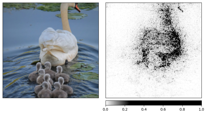
Attribution computed using integrated gradients method. Image source: captum.ai

💥 Task 6 💥

Based on example and tutorial, implement attribution with integrated gradients for pre-trained ResNet-34 model used in this laboratory and verify the output on an image after pre-processing.

💥 Task 7 💥

Based on documentation of visualize_image_attr check possible method for visualizing attribution and available options of sign of attributions to visualize. Verify how different values imapct on visualization of attributions.

Consider what positive and negative values mean and how to interpret absolute values in this case.

💥 Task 8 💥

To Integrated Gradients attribution add NoiseTunnel and examine how this method affects the attribution algorithm and the visualization.

💥 Task 9 💥

Based on tutorial Model Interpretation for Pretrained Deep Learning Models, Algorithm Comparison Matrix and Attribution documentation, test and compare 5 different attribution algorithms. Visualize them on a common graph and examine the differences between the outputs of these methods.